Family-Wise Error
Code
library(tidyverse)

theme_set(theme_minimal())

color_primary <- "#2171b5"
color_secondary <- "#888888"
color_reference <- "gray50"
What family-wise error is
A single hypothesis test run at α = .05 has a 5% chance of a false positive when the null hypothesis is true.
Running more than one test on the same data raises the probability that at least one of them turns up significant by chance alone, even though each test still runs at α = .05. The family-wise error rate is the probability of at least one false positive across a set, or family, of tests, all conducted under a true null.
Whether that probability is the right thing to worry about depends on the claim the tests are being used to support.
Claim 1: The treatment affects at least one of multiple outcomes
The first scenario is a claim that holds as soon as any one of several tests comes out significant. It comes up when researchers compare a treatment group to a control group and record multiple outcome measures rather than one, because they don’t know in advance which of them the treatment might affect: the research claim is then that the treatment affects at least one of these outcomes.
Suppose, for illustration, that this claim is false: the treatment affects none of the outcomes, so every one of the comparisons is testing a true null. The claim is wrongly supported whenever at least one of the comparisons is significant by chance. Tracking whether at least one of the first m comparisons is significant, for m = 1 through 20, traces out how often that mistake happens as more outcomes are added.
Code
alpha <- 0.05
k_max <- 20

fwer_any_effect <- tibble(
  m = 1:k_max,
  fwer = 1 - (1 - alpha)^m
)

ggplot(fwer_any_effect, aes(x = m, y = fwer)) +
  geom_line(color = color_primary) +
  geom_point(color = color_primary) +
  scale_y_continuous(labels = scales::percent_format()) +
  labs(x = "Number of outcomes measured (m)", y = "P(claim wrongly asserted)")
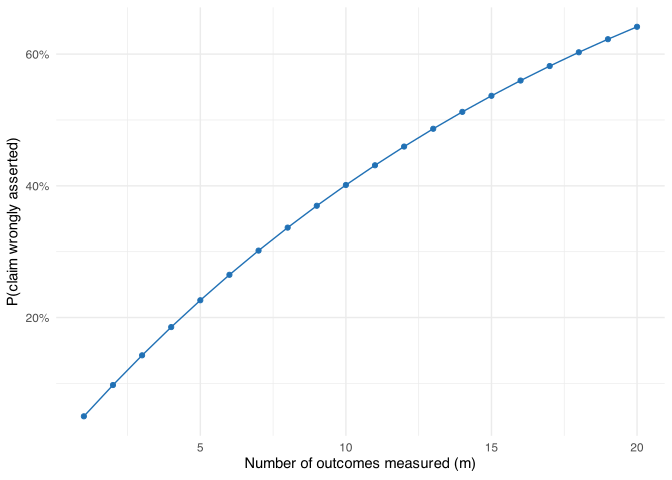
The false-claim rate is 1 - (1 - α)^m. With one outcome measured, it equals α, the per-comparison rate. With five outcomes it has already climbed past 20%; with twenty, past 60%.
The claim here is disjunctive: it is true if the treatment affects at least one outcome, so a false claim requires only one of the m comparisons to be a false positive. That is exactly the family-wise error rate, and it grows with the number of outcomes tested. A claim of this shape needs a correction procedure to keep the false-claim rate near the intended level.
Claim 2: Every condition beats the control
The second scenario is a claim that only holds if every one of several tests comes out significant. In a different study, researchers compare four treatment conditions against a single shared control and claim that every one of the four beats it — four redesigned versions of a product tested against the current baseline, say, with the claim being that all four improve on it. This claim is conjunctive rather than disjunctive: it is only true if every one of the four individual comparisons reflects a real difference, and asserting it means requiring all four p-values to be significant at once.
The simulation below is run across configurations that differ in how many of the four conditions are genuinely identical to control, from all four (a true null throughout) down to none (all four genuinely differ by the same amount), while the rest are drawn with a real effect. Each simulated dataset draws one control sample and reuses it for all four comparisons, matching a shared-control design. For each configuration it records how often all four comparisons are significant at once, both without correction and under a Bonferroni correction that divides α by 4.
Code
set.seed(123)
n <- 40
k <- 4
d <- 0.6
alpha <- .05
n_sim <- 8000

sim_all_beat_control <- map_dfr(0:k, \(n_null) {
  effects <- c(rep(0, n_null), rep(d, k - n_null))

  reps <- map_dfr(seq_len(n_sim), \(i) {
    control <- rnorm(n, 0, 1)
    ps <- map_dbl(effects, \(delta) {
      treatment <- rnorm(n, delta, 1)
      t.test(treatment, control)$p.value
    })
    tibble(
      Uncorrected = all(ps < alpha),
      Corrected = all(ps < alpha / k)
    )
  })

  tibble(
    n_null = n_null,
    Uncorrected = mean(reps$Uncorrected),
    Corrected = mean(reps$Corrected)
  )
})

sim_all_beat_control
| n_null | Uncorrected | Corrected |
|---|---|---|
| 0 | 0.490375 | 0.245375 |
| 1 | 0.028000 | 0.006000 |
| 2 | 0.004875 | 0.000250 |
| 3 | 0.002625 | 0.000375 |
| 4 | 0.001250 | 0.000125 |
sim_all_beat_control_long <- sim_all_beat_control |>
  pivot_longer(
    c(Uncorrected, Corrected),
    names_to = "method",
    values_to = "rate"
  )

ggplot(sim_all_beat_control_long, aes(x = n_null, y = rate, color = method)) +
  geom_line() +
  geom_point() +
  geom_hline(yintercept = alpha, linetype = "dashed", color = color_reference) +
  scale_color_manual(
    values = c("Uncorrected" = color_primary, "Corrected" = color_secondary)
  ) +
  labs(
    x = "Number of the 4 conditions that are truly identical to control",
    y = "P(all 4 comparisons significant)",
    color = NULL
  )
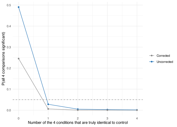
The right-hand side of the plot is where the claim is false: at least one of the four conditions doesn’t really differ from control, so asserting “all four beat control” would be a mistake. Making that mistake requires the one (or more) truly null comparisons to come up significant by chance while the genuinely different conditions also come up significant. Requiring more from the compound event only makes it less likely, not more, so the uncorrected false-claim rate stays at or below α across every one of these configurations without any correction at all.
The left-hand side, at zero truly null conditions, is where the claim is true: all four conditions really do differ from control. There, the value on the y-axis is the power to correctly assert the claim, not an error rate, and this is where the two methods pull apart. The uncorrected procedure has substantially more power to detect the true conjunction than the Bonferroni-corrected one, because the correction applies a stricter threshold on all four comparisons even though the false-claim rate was already controlled without it.
A claim that only holds when every one of several comparisons holds is called an intersection-union test. Using each comparison at the uncorrected level α already keeps the overall false-claim rate at or below α, regardless of how many comparisons are involved or how correlated they are with each other. Correcting for multiplicity here trades power for protection the claim never needed.
Claim 3: Which of the outcomes does the treatment affect?
The third scenario sits between the first two. A researcher measures many outcomes, tests each one, and reports the subset that came out significant as the outcomes the treatment affected. The claim is not that at least one outcome is affected, and not that all of them are. It is a claim about the membership of the reported set, asserted separately for each outcome the set contains.
A single false positive does not sink a claim of this shape the way it sinks the disjunctive claim of the first scenario, because the other genuine discoveries still stand. But multiplicity cannot be ignored the way it can for the conjunctive claim of the second, because each outcome in the set is asserted on its own and each one can be wrong. What matters is how large a fraction of the reported set is wrong. The relevant quantity is the false discovery rate: the expected proportion of false positives among the outcomes flagged as significant, counting the proportion as zero when nothing is flagged.
This is a different target from the family-wise error rate. The family-wise error rate asks whether there is any false positive at all; the false discovery rate asks what share of the flagged outcomes are false. When a researcher screens twenty outcomes expecting to follow up on the hits, one false positive among ten genuine discoveries is a very different situation from one false positive and nothing else, and the family-wise error rate treats them the same.
The simulation below measures twenty outcomes and varies how many of them are truly identical to control, from none up to all twenty, drawing the rest with a real effect of the same size. For each simulated dataset it tests all twenty comparisons and forms a reported set three ways: uncorrected, with each comparison at α; Bonferroni, which divides α by twenty and controls the family-wise error rate; and Benjamini-Hochberg, which controls the false discovery rate at a target level q. For each configuration it records the false discovery rate and the proportion of the truly affected outcomes that end up flagged.
Code
set.seed(123)
n <- 40
k <- 20
d <- 0.6
q <- .05
n_sim <- 2000

sim_which_outcomes <- map_dfr(seq(0, k, by = 4), \(n_null) {
  is_null <- c(rep(TRUE, n_null), rep(FALSE, k - n_null))
  effects <- ifelse(is_null, 0, d)

  reps <- map_dfr(seq_len(n_sim), \(i) {
    ps <- map_dbl(effects, \(delta) {
      control <- rnorm(n, 0, 1)
      treatment <- rnorm(n, delta, 1)
      t.test(treatment, control)$p.value
    })

    flag <- function(reject) {
      tibble(
        fdp = sum(reject & is_null) / max(1, sum(reject)),
        tdr = sum(reject & !is_null) / max(1, sum(!is_null))
      )
    }

    bind_rows(
      flag(ps < q) |> mutate(method = "Uncorrected"),
      flag(ps < q / k) |> mutate(method = "Bonferroni"),
      flag(p.adjust(ps, "BH") < q) |> mutate(method = "Benjamini-Hochberg")
    )
  })

  reps |>
    group_by(method) |>
    summarize(fdr = mean(fdp), power = mean(tdr), .groups = "drop") |>
    mutate(n_null = n_null)
})
sim_which_outcomes |>
  filter(method %in% c("Uncorrected", "Benjamini-Hochberg")) |>
  ggplot(aes(x = n_null, y = fdr, color = method)) +
  geom_line() +
  geom_point() +
  geom_hline(yintercept = q, linetype = "dashed", color = color_reference) +
  scale_y_continuous(labels = scales::percent_format()) +
  scale_color_manual(
    values = c(
      "Benjamini-Hochberg" = color_primary,
      "Uncorrected" = color_secondary
    )
  ) +
  labs(
    x = "Number of the 20 outcomes that are truly identical to control",
    y = "False discovery rate",
    color = NULL
  )
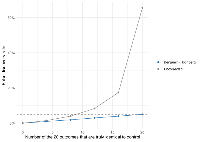
Without correction, the false discovery rate climbs well past the target as more of the outcomes are truly null, because each null outcome contributes its own 5% chance of a false positive to the reported set. Benjamini-Hochberg holds the false discovery rate at or below q across every configuration. Where there are no true effects at all, at the far right, it coincides with the family-wise error rate, since any single false positive then makes the entire reported set false.
Controlling the false discovery rate is not the same as controlling the family-wise error rate, and Bonferroni does the latter. The question is what that stricter control costs in true discoveries.
sim_which_outcomes |>
  filter(method %in% c("Bonferroni", "Benjamini-Hochberg"), n_null < k) |>
  ggplot(aes(x = n_null, y = power, color = method)) +
  geom_line() +
  geom_point() +
  scale_y_continuous(labels = scales::percent_format()) +
  scale_color_manual(
    values = c(
      "Benjamini-Hochberg" = color_primary,
      "Bonferroni" = color_secondary
    )
  ) +
  labs(
    x = "Number of the 20 outcomes that are truly identical to control",
    y = "Proportion of true effects flagged",
    color = NULL
  )
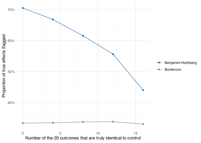
When many of the outcomes carry a real effect, Benjamini-Hochberg flags substantially more of them than Bonferroni does, because its threshold relaxes as more small p-values appear. As the number of true effects shrinks, the gap narrows: with fewer genuine effects among many null outcomes, there is less for the relaxed threshold to work with, and Benjamini-Hochberg moves toward Bonferroni. The gain from targeting the false discovery rate is largest exactly when it matters most, when there are many real effects to be found.
The identification claim calls for controlling the false discovery rate, not the family-wise error rate. Bonferroni guards against any false positive at all, which is stricter than a claim about the membership of a set requires, and it pays for that strictness in missed true effects. Benjamini-Hochberg controls the quantity the claim actually puts at risk, the fraction of the reported set that is false, and recovers much of the lost power in return.
What counts as a “family”
The formula from the first scenario takes one input: m, the number of tests in the family. Deciding what belongs in that family is a judgment call, not something the data can settle.
A family is usually understood as the set of tests that address one research question or one claim. The 20 outcome comparisons in the first scenario are a natural family, since a reader would treat “the treatment did something” as one claim regardless of which specific outcome carries it. A comparison reported in an unrelated part of the same paper, addressing a different question with different data, is ordinarily a separate family: correcting across it would control an error rate that has no shared claim behind it.
The boundary gets harder to draw with secondary or exploratory comparisons. A study with one pre-registered primary outcome and ten additional outcomes examined without a specific prior hypothesis raises the question of whether the primary test stands alone or belongs to a family of eleven. Two researchers can look at the same set of analyses and disagree about how many families it contains, because the answer depends on what claim each analysis is being used to support, not on any property of the data itself.
When to correct and when not to
A single planned comparison, specified before the data were seen and used to answer one question, is a family of one. The formula from the first scenario gives a family-wise error rate equal to α in that case, so there is nothing for a correction to do.
Beyond that, whether a family needs correction, and what kind, depends on the shape of the claim, not just the number of comparisons in it. A disjunctive claim — true if any one comparison shows an effect, as in the first scenario — is put at risk by a single false positive, and the false-claim rate climbs with the number of comparisons exactly as the family-wise error rate does. A conjunctive claim — true only if every comparison shows an effect, as in the second scenario — is protected by its own structure: making the compound claim requires every comparison to come out significant, and that requirement can only lower the chance of a false claim, never raise it. An identification claim — asserting which specific comparisons hold, as in the third scenario — needs correction too, but aimed at the false discovery rate rather than the family-wise error rate, because what is at risk is the fraction of the reported set that is wrong rather than the presence of any single false positive. The conjunctive claim is the one that needs no correction at all.
Even where correction is warranted, it is a trade, not a free improvement: holding the family-wise error rate at α means using a stricter threshold for each individual test, which lowers the power to detect a real effect on any one of them. Whether that trade is worth making depends on the cost of a false positive relative to the cost of missing a true effect in the context at hand. A confirmatory result that will inform a costly downstream decision usually calls for tighter control; an early, exploratory scan intended to generate candidates for later, better-powered follow-up can tolerate a higher family-wise error rate in exchange for more power to notice something worth pursuing.
The omnibus F-test page works through this trade-off concretely for the case of pairwise comparisons following an ANOVA, comparing an uncorrected procedure against Holm and Tukey correction under a partial null.