The Omnibus F-Test
Code
library(tidyverse)

theme_set(theme_minimal())

color_primary <- "#2171b5"
color_secondary <- "#888888"
color_reference <- "gray50"

set.seed(42)
n <- 50
n_sim <- 1000
What it is
The omnibus F-test is the overall significance test in a one-way ANOVA. Its null hypothesis is that all group means are equal; the alternative is that at least one pair of means differs, without specifying which.
The LSD procedure
Fisher’s Least Significant Difference (LSD) procedure uses the omnibus F-test as a gate: if it rejects, follow up with uncorrected pairwise t-tests; if not, stop. The claim is that the gate provides enough protection that the follow-up tests don’t need their own correction. Whether that holds depends on the number of groups.
k = 2
With two groups there is only one pairwise comparison, so multiplicity is not a concern. The omnibus F-test with two groups is algebraically equivalent to a two-sample t-test, and LSD reduces to that single test.
k = 3
Three groups give three pairwise comparisons. Under a partial null — two groups with equal means, one different — there is exactly one null pair. The following simulation uses groups A and B at μ = 0 and group C at μ = 0.5, measuring the familywise error rate on the null pair (A vs. B) under LSD and Holm correction.
Code
sim_k3 <- map_dfr(seq_len(n_sim), \(i) {
  A <- rnorm(n, 0.0, 1)
  B <- rnorm(n, 0.0, 1)
  C <- rnorm(n, 0.5, 1)

  data_k3 <- bind_rows(
    tibble(group = "A", y = A),
    tibble(group = "B", y = B),
    tibble(group = "C", y = C)
  )

  omnibus_p <- oneway.test(y ~ group, data = data_k3, var.equal = TRUE) |>
    pluck("p.value")

  pairs_df <- tibble(
    pair = c("A-B", "A-C", "B-C"),
    raw_p = c(
      t.test(A, B) |> pluck("p.value"),
      t.test(A, C) |> pluck("p.value"),
      t.test(B, C) |> pluck("p.value")
    )
  ) |>
    mutate(holm_p = p.adjust(raw_p, "holm"))

  null_raw_p <- filter(pairs_df, pair == "A-B") |> pull(raw_p)
  null_holm_p <- filter(pairs_df, pair == "A-B") |> pull(holm_p)

  tibble(
    gate_error = omnibus_p < .05 && null_raw_p < .05,
    holm_error = null_holm_p < .05
  )
})

sim_k3 |>
  summarise(
    `LSD` = mean(gate_error),
    `Holm correction` = mean(holm_error)
  ) |>
  pivot_longer(everything(), names_to = "Method", values_to = "FWER")
| Method | FWER |
|---|---|
| LSD | 0.042 |
| Holm correction | 0.027 |
LSD holds the familywise error rate at or below α. Hayter (1986) proved this holds in general for k = 3: with only one null pair, the omnibus rejects because of the real difference, and that does not increase the false positive rate on the null pair.
k ≥ 4
With four or more groups, the partial null can include multiple null pairs alongside real differences. Four groups with means 0, 0, 0.5, and 0.5 give four pairs with real differences and two genuinely null pairs (A vs. B and C vs. D). The simulation compares LSD against Holm correction and Tukey HSD on those null pairs.
Code
sim_k4 <- map_dfr(seq_len(n_sim), \(i) {
  A <- rnorm(n, 0.0, 1)
  B <- rnorm(n, 0.0, 1)
  C <- rnorm(n, 0.5, 1)
  D <- rnorm(n, 0.5, 1)

  data_k4 <- bind_rows(
    tibble(group = "A", y = A),
    tibble(group = "B", y = B),
    tibble(group = "C", y = C),
    tibble(group = "D", y = D)
  )

  omnibus_p <- oneway.test(y ~ group, data = data_k4, var.equal = TRUE) |>
    pluck("p.value")

  pairs_df <- tibble(
    a = c("A", "A", "A", "B", "B", "C"),
    b = c("B", "C", "D", "C", "D", "D"),
    raw_p = c(
      t.test(A, B) |> pluck("p.value"),
      t.test(A, C) |> pluck("p.value"),
      t.test(A, D) |> pluck("p.value"),
      t.test(B, C) |> pluck("p.value"),
      t.test(B, D) |> pluck("p.value"),
      t.test(C, D) |> pluck("p.value")
    )
  ) |>
    mutate(holm_p = p.adjust(raw_p, "holm"))

  tukey_p <- TukeyHSD(aov(y ~ group, data = data_k4))$group[
    c("B-A", "D-C"),
    "p adj"
  ]

  null_p <- filter(pairs_df, (a == "A" & b == "B") | (a == "C" & b == "D"))

  tibble(
    gate_error = omnibus_p < .05 && any(pluck(null_p, "raw_p") < .05),
    holm_error = any(pluck(null_p, "holm_p") < .05),
    tukey_error = any(tukey_p < .05)
  )
})

sim_k4 |>
  summarise(
    `LSD` = mean(gate_error),
    `Holm correction` = mean(holm_error),
    `Tukey HSD` = mean(tukey_error)
  ) |>
  pivot_longer(everything(), names_to = "Method", values_to = "FWER")
| Method | FWER |
|---|---|
| LSD | 0.084 |
| Holm correction | 0.018 |
| Tukey HSD | 0.016 |
LSD inflates the familywise error rate on the null pairs to roughly 10%, double the nominal level. Holm and Tukey both hold it below α without a prior gate. The failure follows directly from the real differences: those effects drive the omnibus to reject on nearly every run, so uncorrected tests proceed regardless, and the null pairs are tested without correction.
Under the complete null, where all group means are equal, LSD controls the FWER for any k. The omnibus rejects about 5% of the time, limiting how often follow-up tests run. The failure only appears when real effects are present, which is the normal situation in which researchers apply the procedure.
The omnibus as a gateway to corrected tests
The more common modern pattern runs the omnibus before applying Holm or Tukey correction. Since correction already controls the familywise error rate, the gate adds no protection that wasn’t already there, and it does not improve power on individual comparisons.
There is one case where reporting both carries information the other doesn’t: when the omnibus is significant but no individual comparison survives correction. That outcome indicates the factor’s effect is diffuse — spread across many pairs with no single comparison large enough to survive pairwise testing. Reporting both results in that case gives the reader information neither alone would convey.
Inconsistency with pairwise results
Using the omnibus as a gate before a pairwise MCP creates a further problem: the two tests can give logically inconsistent results.
The F-statistic summarizes the spread of all k group means into a single test statistic using k-1 numerator degrees of freedom, aggregating signal from every group simultaneously. Tukey compares specific pairs, with a critical value that grows with the number of groups to account for multiple comparisons. Because the two statistics draw on different aspects of the data, they can point in opposite directions.
One direction of disagreement: the omnibus rejects but no pairwise Tukey comparison is significant, including the widest-ranging pair. This can happen when the means are spread across many small differences. The cumulative between-group variance pushes F past its critical value, but no single gap is large enough to clear Tukey’s larger critical value. The gate says to proceed; the MCP finds nothing to report. This outcome is called non-consonance.
The other direction: the omnibus retains but the widest-ranging pair would have been significant under Tukey. When only one pair genuinely differs and the rest are null, those null groups contribute near-zero between-group variance that pulls MSB down, and the concentrated signal in the widest gap is not enough to push F past its critical value. The gate says to stop, but the widest-ranging pair would have been significant had it been tested. This is called incoherence.
Both outcomes make the gate unreliable as a decision rule. Incoherence is the more practically awkward case: the researcher has a result that would survive correction but the gate prevents the test from being run. In practice, researchers in that situation often run the MCP anyway, which means the gate is not controlling the error rate it claims to.
Power for a specific comparison
There is a further cost in statistical power when the research question targets a specific comparison. With four groups where only group 1 has a non-zero mean, the omnibus tests whether any of the four group means differ from one another, while a planned contrast targets group 1 against the remaining three groups directly. The following simulation varies the size of that effect and measures how often each test rejects at α = .05, tracing out power as a function of effect size.
ds <- seq(0, 1, by = 0.05)
n_sim_power <- 5000

sim_power <- map_dfr(ds, \(d) {
  res <- map(seq_len(n_sim_power), \(i) {
    group <- rep(1:4, each = n)
    y <- rnorm(4 * n, c(d, 0, 0, 0)[group], 1)

    aov_fit <- aov(y ~ factor(group))
    omnibus_p <- summary(aov_fit)[[1]]$`Pr(>F)`[1]
    mse <- summary(aov_fit)[[1]]$`Mean Sq`[2]

    lhat <- mean(y[group == 1]) - mean(y[group != 1])
    se_lhat <- sqrt(mse * (1 / n + 1 / (3 * n)))
    contrast_p <- 2 *
      pt(abs(lhat / se_lhat), df = 4 * n - 4, lower.tail = FALSE)

    list(omnibus_sig = omnibus_p < .05, contrast_sig = contrast_p < .05)
  })

  tibble(
    d = d,
    Omnibus = mean(map_lgl(res, "omnibus_sig")),
    Contrast = mean(map_lgl(res, "contrast_sig"))
  )
})

sim_power |>
  pivot_longer(
    c(Omnibus, Contrast),
    names_to = "method",
    values_to = "power"
  ) |>
  ggplot(aes(d, power, color = method)) +
  geom_line(linewidth = 0.8) +
  geom_point(size = 1.5) +
  scale_y_continuous(labels = scales::percent_format()) +
  scale_color_manual(
    values = c("Omnibus" = color_secondary, "Contrast" = color_primary)
  ) +
  labs(x = "Effect size (d)", y = "Power", color = NULL) +
  theme(legend.position = "bottom")
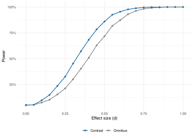
The planned contrast has higher power across the full range of effect sizes. The omnibus simultaneously tests every possible pattern of group differences, which needs three degrees of freedom for four groups and requires a higher critical value at α = .05 than a single-degree-of-freedom test. Two of those degrees of freedom correspond to comparisons among groups 2, 3, and 4 that are null, so they raise the threshold for significance without contributing any signal. The contrast tests only the one relevant comparison with a single degree of freedom, so the full effect in group 1 goes toward clearing a lower bar.
When the omnibus is the right test
The omnibus F-test answers a different question from any pairwise comparison: does this factor explain any variance at all? That is sometimes the scientific question. Fisher developed ANOVA in the context of agricultural experiments with many treatment varieties and no prior theory about which specific varieties would perform better. In that setting the research question is whether fertilizer type matters at all, not whether fertilizer A outperforms fertilizer B. The omnibus tests that factor-level question directly, pooling information across all levels into a single test.
Research questions of this kind still arise. An experiment with many unranked conditions and no specific comparison hypothesized in advance is asking whether the factor matters at all, and the omnibus answers that question directly. In that setting it is not a gateway to something else; it is the test.
Follow-up tests that identify which specific conditions differ still need correction. Real effects drive the omnibus to reject on nearly every run, and uncorrected tests on null pairs inflate the familywise error rate regardless of whether an omnibus preceded them.
Reporting
When specific comparisons with multiple comparison correction are the primary result, the omnibus F is redundant. A significant omnibus says that some pair differs; the corrected comparisons say which and by how much. The exception is the diffuse-effect case: when the omnibus is significant but no corrected comparison is, reporting both gives the reader a result neither alone conveys.
When the omnibus is itself the research question — whether the factor matters at all — it is the primary result and should be reported on its own terms.